[Paper] Neural Collapse

This is a brief review for “Prevalence of neural collapse during the terminal phase of deep learning traing”. You can see the paper at this link.

Overview

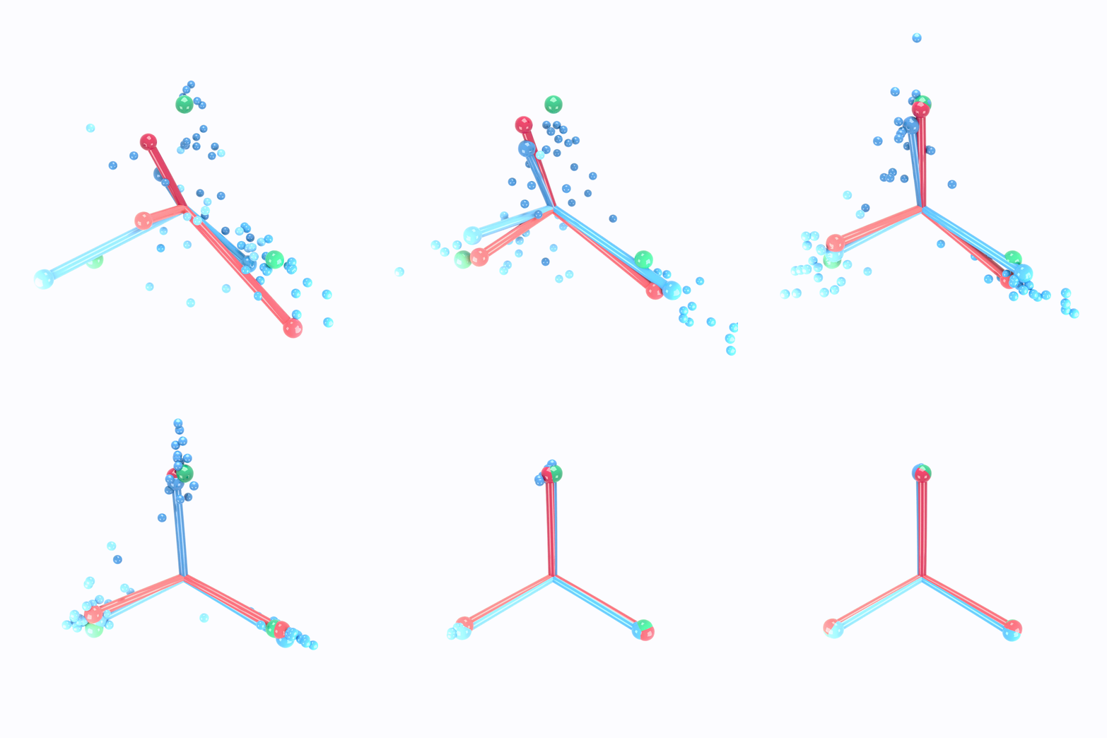
As I know, this is the first paper which introduce the concept of Neural Collapse(NC). This paper highlights an interesting phenomenon which occurs at the end of the training scenario, which is called as terminal phase of training(or TPT). Once the model acheive a good performance or zero error(under decimal points), model shows a kind of collapse at the structure of classifiers! Now, I’d like to introduce the concept and share my insights from it.

We can view the last layer of model as follows:

• Input : activation
• Function : classifier(as a matrix transform)
• Output : Classification $\mathbb{R}^C$

Approach

Process of Neural Collapse(NC)

• NC1: Variablity collapse: within class variation becomes negligible!
  • Activation collapse to their class means
• NC2: Convergence to simplex equiangular tight frame(ETF)
  • class mean vectors converge to a simplex ETF.
  • simplex ETF properties : equal length and equal-sized angles
• NC3: Convergence to self duality
  • class mean vectors and classifier converges to each other.
  • symmetry in classifier decisions!
• NC4: Simplication to nearest class center(NCC)
  • total network choose the nearest class for a given activation(in Euclidean distance)

To be more specific,

1. NC2 implies that mean vectors for each class are “equally spaced” in the feature(activation) space!
   • activation(inputs) are evenly distributed at TPT.
   • In my opinion, this is the results of our loss design!
2. NC implies that linear classifiers(transformation matrix) is equivalent to the set of class mean vectors!

Formations

Notation

$x\in\mathbb{R}^d$ : Input
$h:\mathbb{R}^d\to\mathbb{R}^p$ : Classifier
$h_{i,c}$ : activation for $i$th data in $c$th class
$\mu_{G}=Avg_{i,c} \lbrace h_{i,c} \rbrace \in \mathbb{R}^p$ : Global mean
$\mu_c=Avg_{i}\lbrace h_{i,c}\rbrace \in \mathbb{R}^p$ : class means
$\Sigma_T = Avg_{i,c}\lbrace (h_{i,c}-\mu_G)(h_{i,c}-\mu_G)^T \rbrace \in \mathbb{R}^p \times \mathbb{R}^p$ : total covariance
$\Sigma_B = Avg_{i,c}\lbrace (\mu_{c}-\mu_G)(\mu_{c}-\mu_G)^T \rbrace \in \mathbb{R}^p \times \mathbb{R}^p$ : between class covariance
$\Sigma_W = Avg_{i,c}\lbrace (h_{i,c}-\mu_G)(h_{i,c}-\mu_G)^T \rbrace \in \mathbb{R}^p \times \mathbb{R}^p$: within class covariance
$M = [\mu_c - \mu_G]$
$\dagger$ : Moore-Penrose pseudoinverse

Mathematical description

• NC1 : $\Sigma_W\to 0$
• NC2 :
  
  • $\forall c,c’ \mid \lVert \mu_c - \mu_G\rVert - \lVert \mu_{c’} - \mu_G\rVert \mid \to 0$
  • $<\tilde{\mu_{c}}, \tilde{\mu_{c’}}> \to {C \over C-1} \delta_{c,c’} - {1 \over C-1}$
• NC3:
  • $\lVert {W^T \over \lVert W\rVert } - {M^T \over \lVert M\rVert } \rVert$

Limitation

1. Surely, test results are based on primitive models!
2. Need to be tested on large scale data(Scalability check)
3. It tested on the last layer(activation). For deeper network, we don’t know well.

Insights

According to the author, maybe, classifiers are extremely simple and symmetric!

---

Proposition 1: (Webb and Lowe) Adopting the mean squared error loss in place of cross entropy loss, optimal learnable parameters are given by
$W={1\over C} M^T\Sigma_T^{\dagger}$
$b={1\over C}\mathbb{1} - {1\over C}M^T\Sigma_T^{\dagger}\mu_G $. (Of course, more details are missing!)

Proposition 2: (D. Soudry, E. Hoffer et al.) : TBD

Once we adopt the Proposition 1 with NC1 and NC2, NC3 and NC4 is natural!

Once we adopt the Proposition 2 with NC1 and NC2, NC3 and NC4 is natural! Furthermore, cross entropy loss design maybe constraint on the classifier!

This implies that NC3 and NC4 is accompanied with NC1 and NC2 if we use cross entropy loss! So to speak, inductive bias to NCC exisits in classifier of Proposition 1 and Proposition 2.

---

“Inductive bias” is the reason for the success of deep learning and it can be implicit in training procedure pointing out the Proposition 2 as a foundational results. That is, inductive bias is much more constraining on the outcome than our expectation.

---

In my opinion, the reason why cross entropy loss design has that inductive bias can be explained with update rule!

Softmax layer is commonly used for models used in this paper and the results are used to calculate Cross Entropy loss. When it comes to minimize the loss value, softmax values are also updated so that model enhance the softmax value of true label(class) and lower that of false label. Moreover, softmax value uses dot product which is naturally correlated with cosine similarity. As a result, classifier for the true label is updated to enhance the cosine similarity value. This implies that classifier and input features are aligned with each other which achieve smaller angular distance!

---

Further research

See pepers below here:

• The implicit bias of gradient descent on separable data
• The Optimised Internal Representation of Multilayer Classifier Networks Performs Nonlinear Discriminant Analysis

Explanation of the author X.Y. Han from Operations Research and Information Engineering, Cornel

• Video link